Difference between moving multiple axes using CAM profiles or interpolation

In a CAM profile the axes move depending on the position of the master axis, in any direction and whatever its speed / acceleration / deceleration and Jerk.

In an interpolation the axes move according to the speed / acceleration / deceleration / vector Jerk programmed and in the same direction. It would be like the time-based CAM profiles of some controllers, such as the ControlLogix MATC (Motion Axis Time Cam) instruction.

It is explained in detail below.

Operation of a movement by PCAM

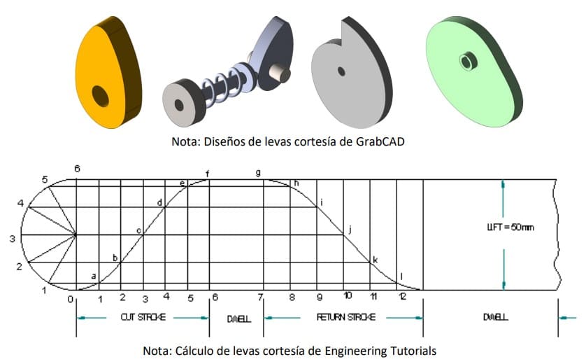
The CAM profiles, also called positioned by tables, electronic cams, PCAM (Position CAM) emulate the movements that have been made by mechanical cams. There are also TCAM (Time CAM) that will be explained later.

The great advantage of electronic cams is that they bring together the good of the mechanical solution and the good of the electronic solution, in other words, they achieve 99% operation like the mechanical and with all the flexibility, for format changes, offered by electronics. This is also what we call Mechatronics.

The main difference with the mechanical cam is its behavior in the event of a power failure, emergency stop or axis failure. Situations in which the position of the slave shaft will be desynchronized to a greater or lesser extent, and it will be necessary to manage it by code to re-synchronize all the axes before restarting production.

When it comes to PCAMs, we always talk about the master axis, which can be a master encoder, it can be a virtual axis, or it can be a program-generated position value and slave axes, which are the ones that will follow the master and are typically real axes, although they can also be virtual.

In the graph at the top right mechanical cams corresponding to valves of an explosion engine are shown, the master shaft rotates the two cams CAM 1 and CAM 2, which are the same, but are out of phase 90º, it is not hard to imagine that, when turning the master axis, the cams will print a vertical movement to the valves (these return through a spring).

Each turning position of the master axis corresponds to a height position to each valve, which will always be the same as the master moves, forward, backward, impulses, it will be impossible for the system to lose synchronism. Moreover, the dynamics of valve movement depends on the movement of the master.

Operation of a movement by PCAM

Given the mechanical system, we are going to convert it to electronic movement, something as “simple” as making a table with the position values that correspond to each slave axis for each degree of rotation of the master (hence the name of positioning by tables in old controllers).

In the current controllers all kinds of interpolations are available, so that with very few values you can already draw the profile, now we will see it with the example in which we will convert the mechanical cams to electronic.

The upper graph (green) shows the variation of the master axis when rotating, a value of 0 to 360º will be produced and return to zero with greater or lesser frequency depending on its rotation speed. Now look at the movement of slave 1 (blue), we see that it reaches a position of 125 mm with a 90º turn of the master and that it returns to 0 with another 90º of the master. And it remains at zero until the end of the cycle, which repeats cyclically

With the types of interpolation offered by the actual controllers to go from one point to another within a profile, this is as easy as setting the values of the four points that we see in yellow in the graph, each point has a value for the master axis (X) and its corresponding value for the slave axis (Y). Each section defined by two points is called a segment, in this case 4 points, 3 segments, its values are P1(X = 0, Y = 0); P2(X=90, Y=125); P3(X=180, Y=0); P2(X=360, Y=0). We will proceed in the same way for slave 2 (orange).

The way in which interpolation calculates intermediate values is with a function according to the type of interpolation chosen, in the example a polynomial of 5º . Once the profiles are defined, the controller reads the position of the master axis and obtains the one that corresponds to the slave, suppose 45º of the master axis to slave 1 (blue) would correspond 62.5 mm that the CPU obtains by applying the function according to the type of interpolation chosen. The position value obtained from the profile is sent directly as a position reference value to the servo drive of the slave axis. In this case we do not talk about speed or acceleration /
deceleration, we look at the position of the master, look for the corresponding position for the slave and send it as a reference, so move as the master axis moves, the slaves will always be in the position that corresponds to them.

Summary / Conclusions of a movement by PCAM

1. A PCAM movement is intended to emulate the movement of a mechanical cam.
2. There is always a position reference source, be it a real, virtual, master encoder or code-generated value and one, or as many as needed, slave axes that will follow the master (each slave would be a cam)
3. The dynamics of the movement of the slave axes depend on that of the master axis, which normally rotates at constant speed, but can also move impulsively or in any other way. In some applications is moved by positioning.
4. With PCAM movements, the most complex applications of synchronized axes, as it could be a rotary cut-off, are solved in a very simple way.
5. The speed / acceleration / deceleration of the slave axis automatically adapts according to that of the master, which contributes to energy efficiency and extends the life cycle of the machine.
6. The most complex part is the generation of the appropriate profile for each axis, by code, starting from the parameters of a format.
7. In 4.0 machines they are used extensively because they offer perfectly synchronized movements regardless of production speed and total flexibility when changing formats.
8. In some applications the master axis, in turn, is moving with a PCAM, allowing almost any physically imaginable movement to be performed.

Operation of a movement by TCAM

TCAM profiles, since the appearance of virtual axes are no longer used and we will find them in few controllers. The difference is that the positions of the slave axis are not a function of the position of the master axis, but of time. As seen in the profile below left and compared with the same but based on PCAM position.

The tables show the values of each point for each profile. To better understand the TCAM, the movement would be the same as if we do it with the PCAM at a master axis speed of 360º/0.45Seg, that is, at a speed of 800 Grad/Seg, but it will not be in synchronism with any axis. In fact, a TCAM is much more like an interpolation movement, which we’ll look at next.

Summary / Conclusions of a movement by TCAM

1. A movement through TCAM aims to perform a positioning whose profile cannot be achieved by “standard” movements.
2. By combining several TCAM movements on several axes, interpolations can be performed.
3. We can also use TCAM if we need the form of the acceleration of a positioning to be one of those that can be achieved with the interpolations between points of the TCAM profile (Ex: sinusoidal)
4. TCAM does not allow to synchronize the slave axes according to the position of the master, for that you have to use PCAM.

How interpolations work.

In a movement by PCAM or TCAM can participate only one slave axis or tens, but in an interpolation a minimum of two axes is required, let’s say the X and Y axis.

In an interpolation the movement of the axes involved is combined (they can be more than two) to get a straight line, an arc, a circle, etc. -for ease of understanding we will assume that we are talking about a table X, Y, as if it were a drawing plotter-. The velocity, acceleration and deceleration is that of the vector resulting from the interpolation, never that of each axis separately.

To perform an interpolation, the Motion profiler does the same as when we graph a function in X, Y

In the example shown in the graph, it is a linear interpolation of the X and Y axes to draw a line from the coordinates X1=10, Y1=10 to X2=60 and Y2=40, so the line has a total distance of ROOT((X2-X1)^2+(X2 X1)^2)= 58.3 mm. The velocity / acceleration / deceleration is referred to this resulting vector.

The first thing to perform the interpolation, the CPU obtains the equation of the line, in this case Y = 3 / 5 X + 4, will apply values to X starting from 10 and up to 60 to each interrupt interval and depending on the programmed dynamic values.

The values of X and Y are sent as a reference position to each servo drive, without any interrelation between both axes, so it is important that the tracking error value is as equal as possible in both.
The graph above shows the path or position of the X and Y axes. In blue, the speeds of each axis and the resulting vector are shown, which is the one we program and the CPU calculates the one that corresponds to each axis.

We can also see the forms of acceleration (green). In the case of a circular interpolation, the process is the same, but with the circumference equation.

Summary / Conclusions of an interpolated movement

1. A motion with interpolations combines the movement of two or more axes to achieve a path in a plane or in space
2. When dynamic values are programmed for motion, they are always referred to the vector resulting from the interpolation.
3. The axes involved in an interpolation have no relationship between them, for this reason it is important to adjust the tracking error of all of them as equally as possible so that the interpolation is as accurate as possible.
4. With interpolation you cannot synchronize axes
5. Using TCAM movements could obtain the same result as with an interpolation, but it would be more complex to program.

Summary / Final conclusions.

1. Modern PAC controllers have all the necessary functionality to solve the vast majority of applications, PCAM, Interpolations and some TCAM. The important thing is to choose the right function depending on the application.
2. If we are clear that axes must be synchronized, devices such as cams or mechanical transmissions, differentials, indexing boxes, etc. must be replaced, without a doubt that it is PCAM.
3. When axes need to combine their movements to make 2D or 3D trajectories and you need to have control of the dynamics of the resulting vector, it is almost certainly interpolations.
4. In some cases (pick & place) the ideal is interpolations for the ease of programming the trajectory, but if the movement must be in synchronism with another machine will have to use PCAM.