Anyone who has not read the TBO magazine (it is an early magazine) will think that setting up a motion control axis (hereinafter CM) has always been as easy as interconnecting all the devices, with prefabricated cables, connecting the bus cables field and from the programming software adjust some parameters, make a self-adjustment and work. At present this is the case, but to reach this point three decades of technological evolution of controllers, servo drives, servo motors and feedback systems have been necessary.
Purpose of the article
In this paper we intend to give a vision of the devices that intervene in the CM, going back to the year 1990. Showing what a typical architecture of an axis was like, how they were adjusted, what benefits they offered, etc. To be able to compare with current systems, after 30 years of evolution and see the great change that this technology has undergone.
Several areas must be differentiated
The CM encompasses three major worlds/areas/fields/or domains. The one known as CNC, for machine tools. The world of robotics and general-purpose applications or GMC in English (General Motion Control). Each of these fields has its peculiarities, for this reason there are specific controls for each area, with different forms of programming, even with different constructive forms. As seen in the following image.

It must also be said that some applications straddle several worlds. For example: In an automatic machine for the manufacture and packaging of wooden slats, with a total of 18 axes, where it turns out that four are for carrying out small milling operations, this would be CNC and the rest for handling, cutting, and packaging, which would be GMC. Clearly the GMC overlaps with the CNC. It must be said that a GMC can also perform such milling, whereas a CNC would find it more difficult to execute the necessary GMC functions. Therefore, in this case we would opt for the GMC.
This article focuses more on the world of General Purpose CM or GMC in English.
First architectures of a GMC system
The graphic shows the typical architecture. The PLC is in charge of controlling the logic of the machine and is the “conductor of the orchestra”, but since it does not have the ability to control axes, it requires an external GMC control, with which it has to communicate, through a handshake by digital I/O, to give the orders to carry out the movements and receive confirmation. On the other hand, it must be communicated to obtain position, velocity, and acceleration values for the movements; In the past, Ethernet field buses were not available and RS-232 or RS-485 communication was common.
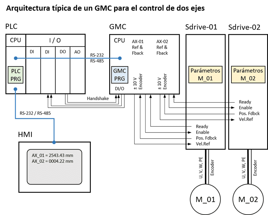
On the other hand, the PLC also communicates with the HMI, which neither had a touch screen nor did it have graphics, to display information on the axes, along with other machine data and to obtain the data entered by the operator.
Regarding the interface of the GMC with the servodrives, it was done by discrete signals; A ±10 V analogue speed or torque reference output signal to the servodrive and a position feedback input, typically incremental, although some equipment already had the option of SSI multiturn absolute feedback, for control of the feedback loop. position. Some digital handshake signals were also needed between the servodrives and the GMC, to control them, a Ready input to know their status and an Enable output to enable power.
At the programming level, several programs had to be developed, one for the PLC and another for the GMC, which worked together synchronized by the handshake signals. A change in the PLC program implied having to also modify the GMC program. which was not very effective. The PLC and GMC programming tools had nothing to do with each other, in many cases the PLC and the GMC were from different manufacturers, so both programs had to be developed in different languages and debugging was not very pleasant.
To put the icing on the cake, the servo drives were analog, and their adjustment was by means of potentiometers, sometimes you had to solder resistors and/or capacitors on pins already arranged for that purpose. This was the part that required the most know-how.
In some cases, the GMC was in the form of a card that was inserted into the PLC backplane, but with no other advantages than eliminating handshake I/O and serial communication for passing parameters, since these communications were carried out using words. I/O over the parallel bus of the backplane.
The early GMC controllers.
The most important element of the GMC is its CPU and at that time only 8-bit microprocessors were available, such as the famous 2.5 MHz Z80 from Zilog or the MOS 6502, which was used in computers such as the Apple I and II, Commodore PET and Nintendo’s Atari 2600 and NES consoles. The first that existed, already 16 bits, was the Intel 8086 at a maximum clock frequency of 5 MHz or the Motorola 68000 that already reached 20 MHz. A bit far from the 64 bits and frequencies of several GHz of today.
There were no flash memories for the firmware, only EPROM memories were available, with maximum capacities of 128 KB. For those who have not read the OBT, these memories could be rewritten with a specific programmer, but to erase them they had to be exposed to UV radiation for about 20 min. And several chips were usually required to contain the firmware of a computer.

To give an example, in this case with a CNC, an OSAI Vector (year 1990) for a milling machine with a total of 5 axes, X, Y, Z and 2 Spindles, the position regulation loop was closed every 10 msec. It had a 4 KB RAM memory, maintained by battery and the math coprocessor occupied four cards full of integrated circuits.
It may even seem implausible to us that a milling machine could machine with the required precision.
Back in 1996, the result of a Joint Venture between Allen Bradley and OSAI, the CNC 7300 with 16 KB of memory and the GMC GP8600 appeared, the latter already designed for general purpose applications, with capacity for xx axes and great functionality, including up to CAM profiles. Other manufacturers also had similar equipment, but I cannot name them due to lack of knowledge of them.
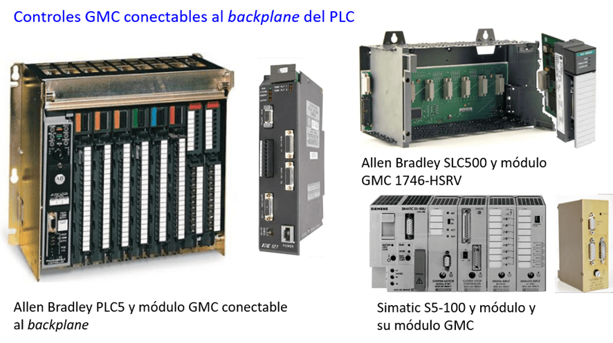
The following image shows the aspect offered by some of the GMC controls, in some you can see the large number of connectors that were required, because all the signals were wired and the servodrives were analog.

Some manufacturers had simple positioners, in the form of cards that were inserted into the PLC backplane, to carry out the most basic operations, such as those shown in the following image.
In this case, the connection between the PLC and the GMC was reduced.
The old servo drives
The offer was quite limited, the best known were those of the manufacturer Indramat, analogue, of course, the adjustments of the regulation loops were made by means of potentiometers and a certain amount of experience was required for their correct operation. First the proportional gain was adjusted to the maximum possible, but without oscillations, then the integral until reaching a minimum error and then the derivative to have a good response to changes in the reference value.

In the TDS (Indramat) equipment, the PID was in the so-called programming module, so that the settings of one equipment could be transferred to another in case of failure of the power part (see image). The servodrive only controlled the speed regulation loop and the current loop, the latter was not accessible, its settings came from the factory. As a speed transducer, tachometric dynamos were used. It must be said that the operation of this equipment was unbeatable, once adjusted correctly, because they are analog, the response is immediate and the resolution “infinite”.
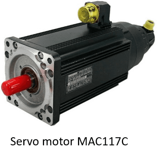
The first brushless servo motors.
Were permanent magnet motors in the rotor. With a tachometric dynamo for regulating the speed loop, plus an encoder and three hall effect sensors (A, B, C) to carry out the phase switching, they typically came mounted in a hybrid of incremental encoder with the three hall sensors, the commutation was trapezoidal because with these sensors only a reading of the rotor position was available every 40 degrees of rotation. The signalsof the incremental encoder were connected to the GMC to close the position loop.
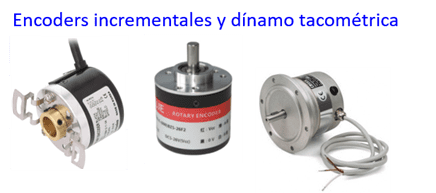
Feedback transducers in the 90s.
As already mentioned, a tachometric dynamo was required to close the speed loop and an AQB-type incremental encoder, with which the GMC closed the position loop.
Normally, each motor manufacturer had hybrid incremental encoders, which already included the signals from the hall sensors for phase switching during power-up.
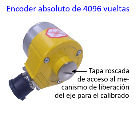
If an absolute feedback system was necessary, there were encoders with multiple optical discs linked by several gears forming a reduction ratio, so that every 8 or 16 turns of the primary disc, a secondary turns one turn and in this way with several reducers and their secondary disks it is possible to count the number of turns. The usual values were from 256 to 1024 counts per turn of the primary and up to 4096 turns could be counted, which made it necessary to transmit up to 22 bits of information.
For this, synchronous serial communication was used, for this reason these encoders were known as SSI (Serial Synchronous Interface) encoders. For its calibration, a threaded cover had to be removed that gave access to a screw that uncoupled the optical discs from the input shaft, so that the discs could be rotated freely, with a special key (similar to a socket wrench) they rotated the discs until the desired reading was obtained, the manufacturer (Steagman, Sick at present) offered a tool that had a small motor and a push button for clockwise rotation and another for anti-clockwise rotation to facilitate the work .
In the CNC world, optical rulers with Sin and Cosine outputs were used, instead of AQB, in order to have a higher resolution.
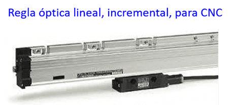
An external module was in charge of dividing the analog signals to be able to generate several points of each period of the sine and cosine, thus increasing the resolution.
Current architecture.
To control an axis, the devices involved remain the same. A controller, a servo drive and a servo motor plus the feedback systems. What has changed a lot is the technology of each of these devices and the architecture of the system.
The most important thing is that a single PAC controller integrates the discipline of CM GMC and that of PLC, so that everything is controlled under the same program, environment and programming language.
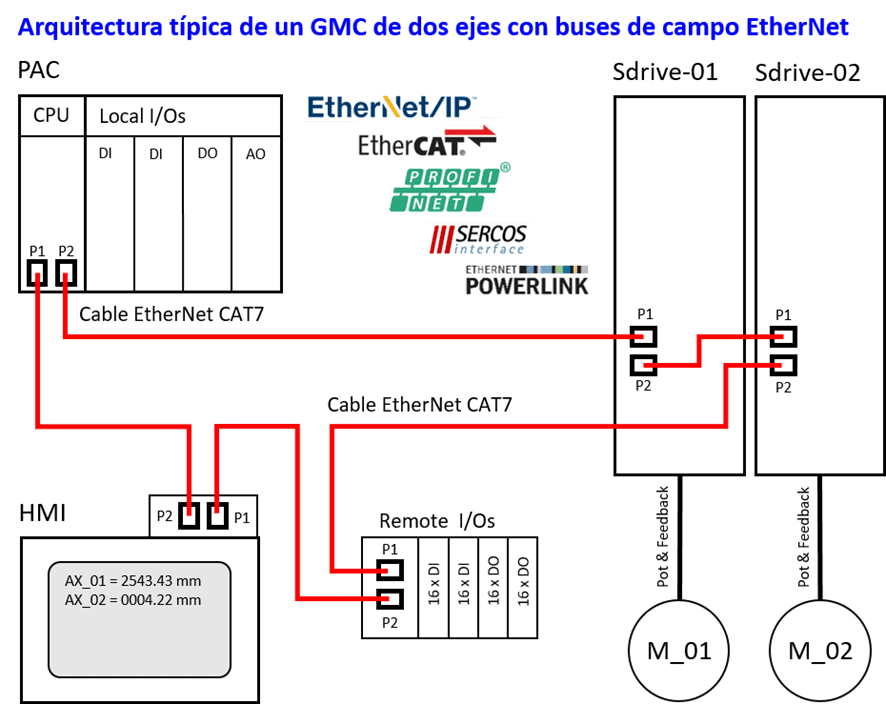
The devices are fully digital and the only interconnection between them is a category 6 or 7 ethernet cable depending on the field bus used, such as EtherNet/IP with CIP Sync, EtherCAT, ProfiNet, SERCOS III or PowerLink. All the I/O functions are carried out via the field bus, which must be synchronous, such as the position reference of the axes and, due to the excess bandwidth, parameters that are not critical in time can be read and written.
Current devices have changed remarkably.
In three decades, many technological changes have taken place, in terms of control we are already in 64-bit CPUs at GHz speeds, in terms of memory it has gone from KB to GBytes, and flash memories appeared that can store GBytes of information and allow immediate firmware upgrades. Hard drives have gone from 20 MBytes to thousands of GBytes and, thanks to solid state drives, their access speed has multiplied. All these advances, more tangible in the IT world, have also benefited industrial control equipment, with the appearance of PACs (Programmable Automation Controllers). You have gone from closing a position loop of an interval of 10 msec. to 0.128 msec. (typical value)

At the servo drive level, the main change has been the transition from analog to digital, from operational amplifiers to DSPs (Digital Signal Processors). Regarding power electronics, the size and losses of IGBTs have been increasingly reduced, and silicon carbide devices, SIC MOSFETs, are even available, which withstand higher temperatures and are still more efficient than IGBTs of Last generation.

Its size has been greatly reduced and double and even triple units are available in the same volume, which allows a large number of axes to be located in a very small space.
At the performance level, current regulation loops incorporate functions to achieve better performance, even though the mechanics have high and/or low frequency resonances and the load suffers notable variations in its inertia.
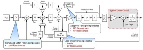
The graph shows the regulation loop diagram of a Rockwell Automation equipment.
Regarding servomotors, there has been a change from a motor with a dynamo plus an encoder and three hall effect sensors, with a power cable, one for the encoder and another for the dynamo, to a motor with a single cable.
The weight / volume / performance ratio has improved dramatically, Cogging, or torque ripple, has been reduced due to the new ways of winding the stator and the arrangement of the magnets in the rotor. Thanks to the current feedback devices, it has been possible to go from a trapezoidal commutation to a sinusoidal one, with all the improvements that this entails.

Endless sizes and types are available, from medium inertia, low inertia, high torque, low RPM motors, known as Direct Torque, or frameless DT, hollow shaft motors, liquid cooled motors , motors for ATEX environments, for the food industry, linear motors in various constructive forms, such as tubular motors. Mechanical actuators with an integrated motor, motors with a mechanical reducer in the same unit, and a host of other options from multiple manufacturers.
Regarding the feedback devices, the advances have also been worth mentioning, there are all kinds of them, the usual incremental ones, incremental ones with Sin/Cos outputs to achieve high resolution, linear rulers, one-turn absolute encoders (essential for sinusoidal phase commutation of synchronous motors), absolute speeds up to 4096 revolutions, with Hiperface, BiSS, EnDat 2.2, EnDat 3 interfaces with functional safety.

And then there are those that already offer direct position information in user units (mm, degrees, inches, etc.) directly, plus much more operational and environmental statistics, via high-speed RS-485 communication. speed, such as DSL – Digital Servo Link, from Sick – or DRIVE-CLiQ from Siemens. The great advantage is that the only connection between the servodrive and the encoder is a simple twisted pair, which goes inside the power cable, thus achieving what is called OCM (One Cable Motor), OCT (One Cable Technology) and the like. according to each manufacturer.
To conclude, the advantages of the latest technology.
Summarized in four paragraphs:
Since the appearance of PACs, the development, debugging, installation, maintenance of CM applications and their continuous improvement have been significantly simplified. In addition, these controllers, day by day, add functions that allow more and more complex applications to be carried out in a relatively easy way, a good example being the calculation of the transforms or kinematics of many robots.
Thanks to synchronous, Ethernet-based fieldbuses, state-of-the-art digital servo drives and their servo motors, what used to require an expert to commission has now become almost transparent, just a basic configuration is enough. of the axis, in some cases a self-adjustment and to work.
If the manufacturer’s installation instructions are followed and its prefabricated cables are used, dozens of axes can be ready and working in one day, lacking “only” the application program. This does not mean that anyone without a minimum base in CM can make applications successfully.
To finish, I dare to say that the latest CM technology is ahead of industry 4.0. there are intelligent transport systems that offer so much that we still do not see how to obtain all their benefits.